ECoG Preprocessing Tutorial with NWB

This tutorial highlights how to preprocess ECoG data which is already stored in a NWB. It will not focus on the low-level preprocessing functions.

Overview of preprocessing steps

• Resampling

• Re-referencing and notch filtering

• Time-frequency power calculation

• Normalizing power for each frequency

Imports

import numpy as np
import matplotlib.pyplot as plt

from pynwb.ecephys import ElectricalSeries

from process_nwb.utils import generate_synthetic_data, generate_nwbfile
from process_nwb.resample import store_resample
from process_nwb import store_linenoise_notch_CAR
from process_nwb.wavelet_transform import store_wavelet_transform

Create and store synthetic neural data

We will create synthetic neural data by convolving white noise with a boxcar, adding power in the high gamma range with modulating amplitude, and adding common line noise (60Hz) with different weights to each channel. We’ll store the raw data in an NWB file and run the preprocessing steps on the file and store the preprocessed data.

num_channels = 64
duration = 10.  # seconds
sample_rate = 10000.  # Hz
new_sample_rate = 500.  # hz

nwbfile, device, electrode_group, electrodes = generate_nwbfile()

Out:

/home/docs/checkouts/readthedocs.org/user_builds/process-nwb/conda/latest/lib/python3.8/site-packages/hdmf/utils.py:577: FutureWarning: DynamicTable.__init__: Using positional arguments for this method is discouraged and will be deprecated in a future major release. Please use keyword arguments to ensure future compatibility.
  warnings.warn(msg, FutureWarning)
/home/docs/checkouts/readthedocs.org/user_builds/process-nwb/conda/latest/lib/python3.8/site-packages/hdmf/utils.py:577: FutureWarning: DynamicTableRegion.__init__: Using positional arguments for this method is discouraged and will be deprecated in a future major release. Please use keyword arguments to ensure future compatibility.
  warnings.warn(msg, FutureWarning)

Storing the data

Now that we have an NWB container, we can generate and store the raw data.

# Create synthetic neural data

neural_data = generate_synthetic_data(duration, num_channels, sample_rate)
t = np.linspace(0, duration, neural_data.shape[0])

ECoG_ts = ElectricalSeries('ECoG_data',
                           neural_data,
                           electrodes,
                           starting_time=0.,
                           rate=sample_rate)
nwbfile.add_acquisition(ECoG_ts)

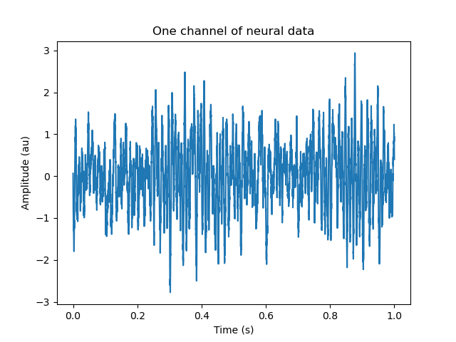
# Here is one chanel of synthetic neural data
plt.plot(t[:10000], neural_data[:10000, 0])
plt.xlabel('Time (s)')
plt.ylabel('Amplitude (au)')
_ = plt.title('One channel of neural data')

Out:

/home/docs/checkouts/readthedocs.org/user_builds/process-nwb/conda/latest/lib/python3.8/site-packages/pynwb/ecephys.py:93: UserWarning: The second dimension of data does not match the length of electrodes. Your data may be transposed.
  warnings.warn("The second dimension of data does not match the length of electrodes. Your data may be "

Preprocessing the data

Now we can follow the steps we would need to do if we were reading a previously recorded and stored dataset in NWB. We’ll first create a preprocessing module where the preprocessed data will be stored.

electrical_series = nwbfile.acquisition['ECoG_data']
nwbfile.create_processing_module(name='preprocessing',
                                 description='Preprocessing.')

rs_data, rs_series = store_resample(electrical_series,
                                    nwbfile.processing['preprocessing'],
                                    new_sample_rate)
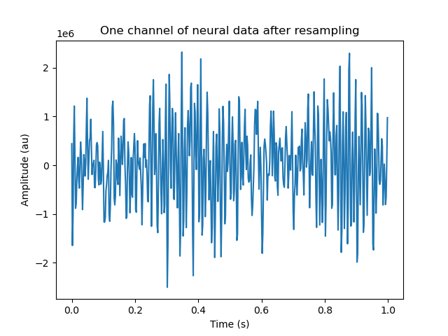
t = np.linspace(0, duration, rs_data.shape[0])

plt.figure()
plt.plot(t[:500], rs_data[:500, 0])
plt.xlabel('Time (s)')
plt.ylabel('Amplitude (au)')
_ = plt.title('One channel of neural data after resampling')
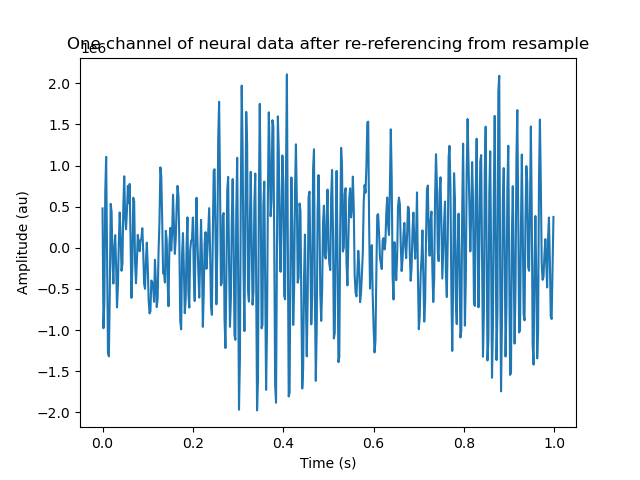
car_data, car_series = store_linenoise_notch_CAR(rs_series,
                                                 nwbfile.processing['preprocessing'])
plt.figure()
plt.plot(t[:500], car_data[:500, 0])
plt.xlabel('Time (s)')
plt.ylabel('Amplitude (au)')
_ = plt.title('One channel of neural data after re-referencing from resample')
tf_data, _ = store_wavelet_transform(car_series,
                                     nwbfile.processing['preprocessing'],
                                     filters='rat',
                                     hg_only=True,
                                     chunked=False)
tf_data = abs(tf_data)

• 
• 

Out:

/home/docs/checkouts/readthedocs.org/user_builds/process-nwb/conda/latest/lib/python3.8/site-packages/pynwb/ecephys.py:93: UserWarning: The second dimension of data does not match the length of electrodes. Your data may be transposed.
  warnings.warn("The second dimension of data does not match the length of electrodes. Your data may be "
/home/docs/checkouts/readthedocs.org/user_builds/process-nwb/conda/latest/lib/python3.8/site-packages/pynwb/ecephys.py:93: UserWarning: The second dimension of data does not match the length of electrodes. Your data may be transposed.
  warnings.warn("The second dimension of data does not match the length of electrodes. Your data may be "
/home/docs/checkouts/readthedocs.org/user_builds/process-nwb/conda/latest/lib/python3.8/site-packages/hdmf/utils.py:577: FutureWarning: DynamicTable.__init__: Using positional arguments for this method is discouraged and will be deprecated in a future major release. Please use keyword arguments to ensure future compatibility.
  warnings.warn(msg, FutureWarning)

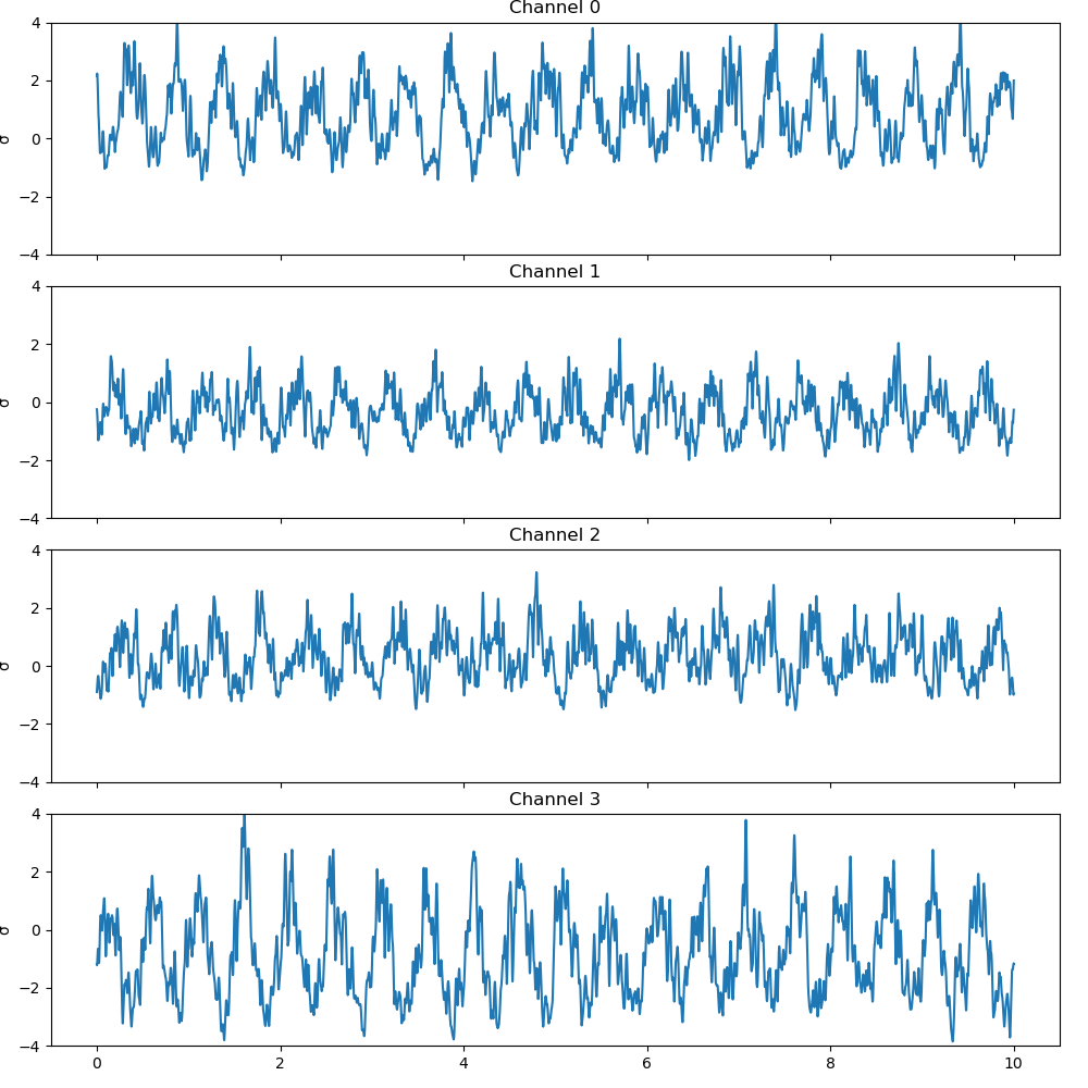
Normalizing power by zscoring

For neural data, power falls off with frequency so it can be difficult to compare amplitude changes across different frequency bands. Furthermore, different electrodes may have different contact with the neural surface, which can lead to meaningless differences in signal amplitude across channels. To address this issue, we normalize each frequency band and electrode by zscoring. In this case, the mean and standard deviation are calculated over the first 0.25 seconds of the signal, our synthetic baseline time. Different experimental recordings and tasks may use different baseline periods.

Then, we will average over the zscored high gamma subbands to form the final high gamma signal the plot the zscored ampliced for all channels.

t = np.linspace(0, duration, tf_data.shape[0])
mean = tf_data[:125].mean(axis=0, keepdims=True)
std = tf_data[:125].std(axis=0, keepdims=True)
tf_norm_data = (tf_data - mean) / std
high_gamma = tf_norm_data.mean(axis=-1)

fig, axs = plt.subplots(4, 1, sharex=True, sharey=True, figsize=(10, 10))
fig.subplots_adjust(hspace=0.4)
fig.tight_layout()

for idx in range(4):
    sig = high_gamma[:, idx]
    axs[idx].plot(t, sig)
    axs[idx].set_title('Channel {0:.0f}'.format(idx))
    axs[idx].set_ylabel('σ')
    axs[idx].set_ylim(-4, 4)

Congrats you now know how to preprocess ECoG signals in NWB!