ECoG Preprocessing Tutorial

This tutorial will go through the common signal processing steps used to preprocess ECoG data from raw voltages to zscored high gamma amplitudes. It will operate on a Numpy array of data rather than use data in an NWB file. All of the steps in this tutorial are typically independent of the experimental task structure.

Overview of preprocessing steps

• Resampling

• Notch filtering

• Re-referencing

• Time-frequency power calculation

• Normalizing power for each frequency

Imports

import numpy as np
import matplotlib.pyplot as plt
from scipy.signal import welch

from process_nwb.utils import generate_synthetic_data
from process_nwb.resample import resample
from process_nwb.linenoise_notch import apply_linenoise_notch
from process_nwb.common_referencing import subtract_CAR
from process_nwb.wavelet_transform import wavelet_transform

Create synthetic neural data

We will create synthetic neural data by convolving white noise with a boxcar, adding power in the high gamma range with modulating amplitude, and adding common line noise (60Hz) with different weights to each channel.

num_channels = 64
duration = 10.  # seconds
sample_rate = 10000.  # Hz
new_sample_rate = 500.  # hz
neural_data = generate_synthetic_data(duration, num_channels, sample_rate) * 1e6
t = np.linspace(0, duration, neural_data.shape[0])[:, np.newaxis]

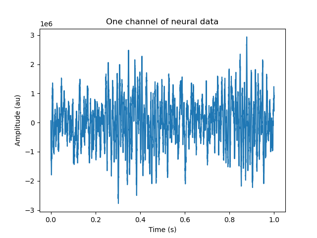
# Here is one chanel of synthetic neural data
plt.plot(t[:10000, 0], neural_data[:10000, 0])
plt.xlabel('Time (s)')
plt.ylabel('Amplitude (au)')
_ = plt.title('One channel of neural data')

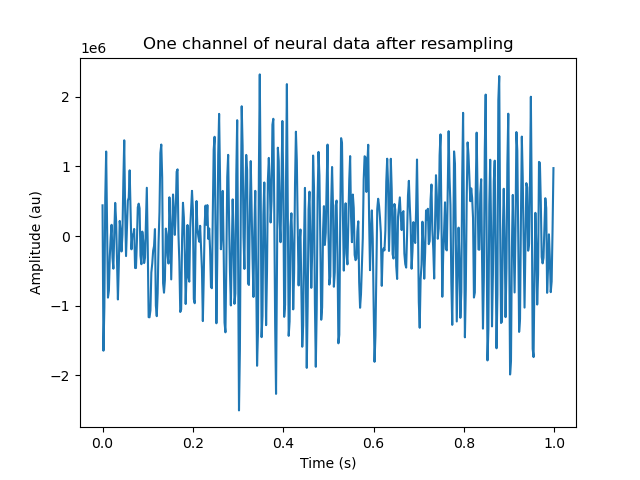
Resampling the data

Often times, the raw data (voltages) are recorded at a much higher sampling rate than is needed for a particular analysis. Here, the raw data is sampled at 10,000 Hz but the high gamma range only goes up to 150 Hz. Resampling the will make many downstream computations much faster.

rs_data = resample(neural_data, new_sample_rate, sample_rate)
t = np.linspace(0, duration, rs_data.shape[0])

plt.plot(t[:500], rs_data[:500, 0])
plt.xlabel('Time (s)')
plt.ylabel('Amplitude (au)')
_ = plt.title('One channel of neural data after resampling')

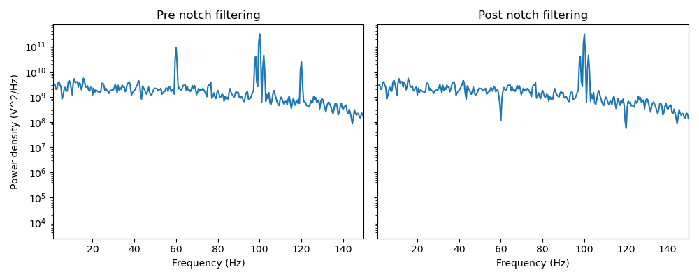
Notch filtering

Notch filtering is used to remove the 60 Hz line noise and harmonics on all channels.

nth_data = apply_linenoise_notch(rs_data, new_sample_rate)

freq, car_pwr = welch(rs_data[:, 0], fs=new_sample_rate, nperseg=1024)
_, nth_pwr = welch(nth_data[:, 0], fs=new_sample_rate, nperseg=1024)

fig, axs = plt.subplots(1, 2, figsize=(10, 4), sharey=True, sharex=True)
axs[0].semilogy(freq, car_pwr)
axs[0].set_xlabel('Frequency (Hz)')
axs[0].set_ylabel('Power density (V^2/Hz)')
axs[0].set_xlim([1, 150])
axs[0].set_title('Pre notch filtering')

axs[1].semilogy(freq, nth_pwr)
axs[1].set_xlabel('Frequency (Hz)')
axs[1].set_xlim([1, 150])
axs[1].set_title('Post notch filtering')
_ = fig.tight_layout()

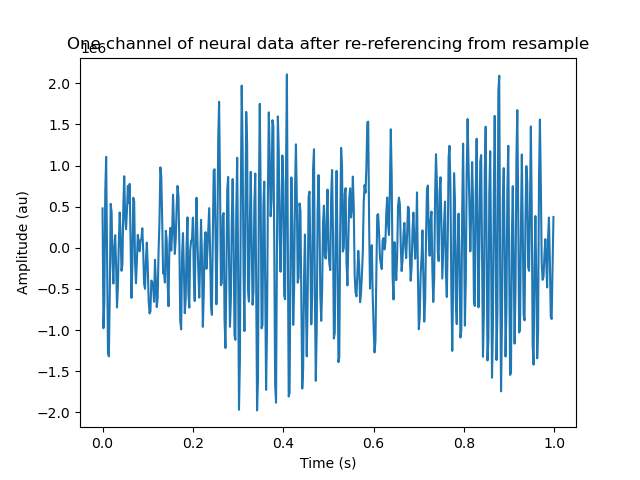
Re-referencing with common average referencing

There is often common noise from neural recording such as movement artifacts or 60 Hz line noise. Additionally, it is often desirable for ECoG channels to be referenced to a common ground. Here, we use a robust estimate of the mean across all channels (for each timepoint). This quantity is then subtracted all channels. By default, this CAR function takes the mean over the center 95% of the electrodes.

car_data = subtract_CAR(nth_data)

plt.plot(t[:500], car_data[:500, 0])
plt.xlabel('Time (s)')
plt.ylabel('Amplitude (au)')
_ = plt.title('One channel of neural data after re-referencing from resample')

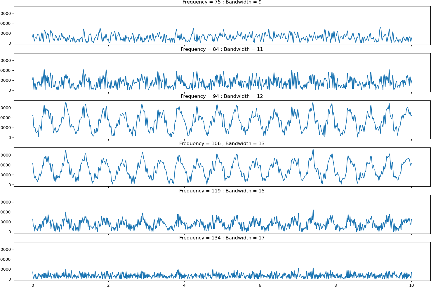
Time-frequency decomposition with wavelets

Here we decompose the neural time series into 6 different frequency subbands in the high gamma range using a wavelet transform. The wavelet transform amplitude is complex valued and here we take the absolute value.

Note how the bands with center frequency nearest 100 Hz have larger amplitude.

tf_data, _, ctr_freq, bw = wavelet_transform(car_data, new_sample_rate,
                                             filters='rat', hg_only=True)
# Z scoring the amplitude instead of the complex waveform
tf_data = abs(tf_data)

num_tf_signals = len(ctr_freq)
fig, axs = plt.subplots(num_tf_signals, 1, sharex=True, sharey=True, figsize=(15, 10))
fig.subplots_adjust(hspace=0.4)
fig.tight_layout()


for idx in range(num_tf_signals):
    sig = tf_data[:, 0, idx]
    axs[idx].plot(t, sig)
    axs[idx].set_title('Frequency = {0:.0f} ; Bandwidth = {1:0.0f}'.format(ctr_freq[idx], bw[idx]))
    axs[idx].set_ylabel('Amp. (au)')

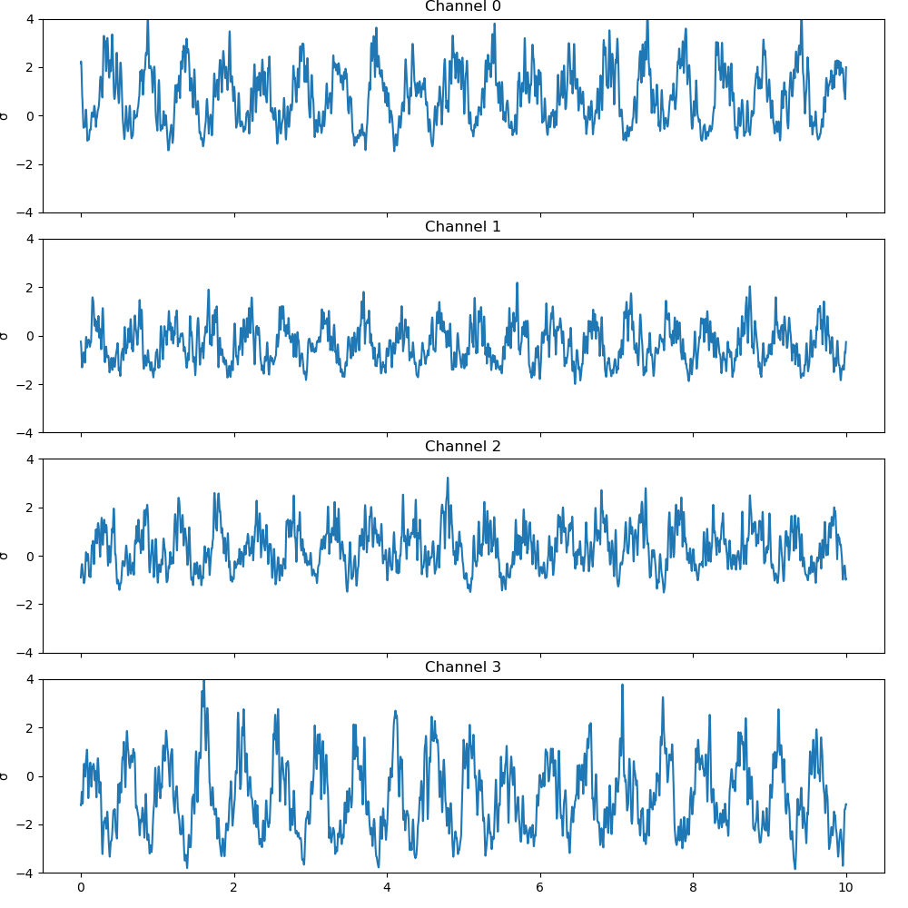
Normalizing power by zscoring

For neural data, power falls off with frequency so it can be difficult to compare amplitude changes across different frequency bands. Furthermore, different electrodes may have different contact with the neural surface, which can lead to meaningless differences in signal amplitude across channels. To address this issue, we normalize each frequency band and electrode by zscoring. In this case, the mean and standard deviation are calculated over the first 0.25 seconds of the signal, our synthetic baseline time. Different experimental recordings and tasks may use different baseline periods.

Then, we will average over the zscored high gamma subbands to form the final high gamma signal the plot the zscored ampliced for all channels.

mean = tf_data[:125].mean(axis=0, keepdims=True)
std = tf_data[:125].std(axis=0, keepdims=True)
tf_norm_data = (tf_data - mean) / std
high_gamma = tf_norm_data.mean(axis=-1)

fig, axs = plt.subplots(4, 1, sharex=True, sharey=True, figsize=(10, 10))
fig.subplots_adjust(hspace=0.4)
fig.tight_layout()

for idx in range(4):
    sig = high_gamma[:, idx]
    axs[idx].plot(t, sig)
    axs[idx].set_title('Channel {0:.0f}'.format(idx))
    axs[idx].set_ylabel('σ')
    axs[idx].set_ylim(-4, 4)

Congrats you now know how to preprocess ECoG signals!